Taqi Shah Blogspot

I will start by talking about the most basic solution to search problems, which are an integral part of artificial intelligence.

What the hell are search problems?

In simple language, search problems consist of a graph, a starting node and a goal(also a node). Our aim while solving a search problem is to get a path from the starting node to the goal.

Consider the diagram below, we want to get to the node G starting from the node S.

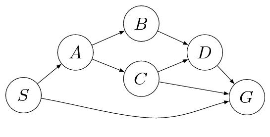
Which path will we get on solving the search problem? How do we get the path? This is where algorithms come into picture and answer all our questions! We will look at Depth First Search which can be seen as a brute force method of solving a search problem.

Creating the search tree

So how do we simplify this problem? If we reduce the graph structure to a tree(not particularly a binary tree!), the problem would be to find a node with a particular value starting from the root.

So the tree would be as follows:

S will be the root of the tree. S will have children A and G. A will have children B and C. B will have only one child D. C will have children D and G. D will have only one child G.

Now you may ask which ‘D’ will have the child G, the one which is the child of B or the one which is a child of C? The answer is both. We want to consider all the possibilities and thus we have to show all the connections uniquely in the tree.

The diagram below shows the created search tree. Note that the nodes are alphabetically taken from left to right. This will be important later!

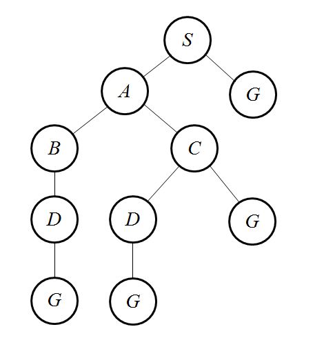
Also note that all the leaf nodes are G. This is not because G is the goal, but because there are no edges originating from G. Even if your goal was say D, the search tree would have remained the same.

Depth first search

Now solving the problem is just a matter of generalizing binary tree search to a tree which does not have a fixed number of children in each of its nodes. Depth First Search is quite similar to preorder traversal of a binary tree where you look at the left child, then the node itself and then the right child.

In Depth First Search, there is a priority queue where each element is a path from the root of the tree. The priority of an element is the number of nodes in the path. Higher the number, higher the priority. We use this priority queue in the following algorithm:

Insert the root node into the priority queue
While the queue is not empty
      Dequeue the element with highest priority
      (In case the priorities are same, the alphabetically smaller element is chosen)
      If the path is ending in the goal state, print the path and exit
      Else
            Insert all the children of the dequeued element, into the queue

Now let us apply the algorithm on the above tree and see what it gives us. We will write down the state of the priority queue at each iteration and look at the final output. Each element of the queue is written as [path,priority].

Initialization: { [ S , 1 ] }
Iteration1: { [ S->A , 2 ] , [ S->G , 2 ] }
Iteration2: { [ S->A->B , 3 ] , [ S->A->C , 3 ] , [ S->G , 2 ] }
Iteration3: { [ S->A->B->D , 4 ] , [ S->A->C , 3 ] , [ S->G , 2 ] }
Iteration4: { [ S->A->B->D->G , 5 ] , [ S->A->C , 3 ] , [ S->G , 2 ] }

Iteration5 gives the final output as S->A->B->D->G.

There are many things worth mentioning here:
-> The creation of the search tree is not a part of the algorithm. It is used only for visualization.
-> The algorithm returns the first possible path encountered, it does not search for all possible paths.
-> The returned path is the leftmost possible path in the search tree.

It searches deep into the leftmost branch first, and hence the name Depth First Search.

Because of the above properties, Depth First Search is not favored in not most cases. For example, if we need the shortest path Depth First Search won’t serve our purpose as it will return S->A->B->D->G instead of S->G. This is where Breadth First Search comes into picture. We shall see that in the next post!

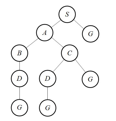
In this post I will talk about the Breadth First Search algorithm for solving a search problem. Given below are the diagrams of the example search problem and the created search tree. If you don’t know what search problems are and how search trees are created visit this post.

Breadth First Search

Breadth First Search is a great algorithm for getting the shortest path to your goal(not applicable to graphs which have weights assigned to edges). Breadth First Search by the name itself suggests that the breadth of the search tree is expanded fully before going to the next step.

Now unlike Depth First Search we don’t need a priority queue for this. We use two queues instead, one for expanding and one for temporary storing. Again each element of the queue is a path from the root of the tree. The algorithm using these queues is the following:

Insert the root into the expanding queue
While expanding queue is not empty
      Copy contents of expanding queue to temporary queue
      Empty the expanding queue
      For each node in the temporary queue
            Dequeue one element from the temporary queue
            If the path is ending in the goal state, print the path and exit
            Else
                  Insert all the children of the dequeued element into the expanding queue

Now let us apply the algorithm on the above tree and see what it gives us. We will write down the state of the expanding queue at each iteration and look at the final output. Each element of the queue is written as [path].

Initialization: { [ S ] }
Iteration1: { [ S->A ] , [ S->G ] }
Iteration2 gives the final output as S->G.

Things worth mentioning:

->The creation of the search tree is not a part of the algorithm. It is only for visualization.
->The algorithm returns the first possible path encountered(in this case optimal), it does not search for all possible paths.
->The returned path is the shortest possible path in the search tree.

It searches the tree level by level, i.e. expands all possible paths till each node at a particular height and then goes for the level below. Thus it is rightly called Breadth First Search. This also explains why we did not require the priority queue used in Depth First Search. Remember that the priority of each element was the number of nodes that the path contained. Here, each element has the same number of nodes since we are expanding level by level, and thus having a priority does not make sense.

I mentioned before that Breadth First Search is not optimal for graphs having weights assigned to edges. An example of such a graph is given below:

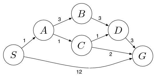
For this example Breadth First Search will return the path as S->G whereas the path having minimum cost associated with it is S->A->C->G. Thus Breadth First Search returns the path shortest in length and not optimal in cost. We shall solve this problem by using Uniform Cost Search in the next post!

Search heuristics are important in improving the efficiency of a search problem. This post will describe what heuristics are and why they are used in artificial intelligence applications. I will cover some of the standard topics in heuristics which are admissible and consistent heuristics.

What are heuristics?

Heuristics can be said to be estimates of how far the goal state is. Heuristics basically predict how far the goal state maybe or how much it will cost to get to the goal state from a particular node. Now the question that arises is, when we know the cost of getting to the goal state from every node why do we have to search at all? We don’t know the cost of getting to the goal state, we have an estimate or prediction for it which may or may not be correct.

Let us take an example to demonstrate how we can estimate costs of reaching a goal state. Consider the maze below:

Let the opening at the left of the maze be the start state, and the one at the top be the goal state. We consider the maze to be split into blocks having (x,y) co-ordinates, with the width of a path being 1 block. It is quite difficult for us to say how many steps a person may have to move to get to the goal state, since we will have to solve the search problem to find that. It makes no sense to solve a search problem to find out a heuristic, since heuristics are meant for the efficient solving of search problems.

Now imagine the maze without any walls or obstacles. What would be the shortest path then? It would be a steps to the right and b steps to the top. This is called the Manhattan distance between two points and can be used as a heuristic for the given maze. Another obvious heuristic is the Euclidean distance between the two points.

It can also be clearly seen that heuristics don’t give the actual cost of the path. In this particular example, if we use the Euclidean distance as a heuristic, there are points that are far from the goal state as compared to the start state, but the actual cost of getting to the goal state from these points is smaller than the actual cost from the start state.

Admissible Heuristics

A heuristic is said to be admissible if the value of the heuristic is always smaller than or equal to the actual cost of getting to the goal state.

Consistent Heuristics

A heuristic is said to be consistent if the heuristic value for every edge is smaller than or equal to the actual cost of the edge. The heuristic value for an edge might be defined as h(AB) = h(A) – h(B). The heuristic of an edge AB is the heuristic value at A minus the heuristic value at B.
It is an obvious statement to say that if a heuristic is consistent then it is also admissible.

Let us take the following diagram as an example for admissible and consistent heuristics:

Clearly h1 is an admissible heuristic. But it is not consistent since the heuristic value for edge SA is 2 whereas the true value is 1. Also h2 is both admissible as well as consistent.